15 Advanced Forecasting Models: Exponential Smoothing (ETS)
Now that we have established our performance baselines with simple models, we are ready to explore the sophisticated forecasting workhorses that can capture the complex patterns we identified during our exploratory analysis. These advanced models automatically detect and model the trends, seasonality and other temporal structures that make our time series predictable.
The true power of the fable framework shines here - what traditionally required extensive statistical expertise and manual parameter tuning is now accessible through intuitive, automated functions that maintain the tidy workflow we have built throughout this book.
ETS models are remarkably powerful yet intuitive. They work by assigning exponentially decreasing weights to historical observations, with more recent data receiving higher importance. Imagine you are trying to predict tomorrow’s temperature. You would probably give more weight to today’s temperature than to last week’s, and even more weight to this morning’s reading.This intuitive approach is the beautiful simplicity behind Exponential Smoothing.
The magic of ETS lies in its elegant balance: It is sophisticated enough to capture complex patterns yet transparent enough that you can understand exactly what it is doing.
15.1 The Core Intuition: Why “Exponential” Smoothing?
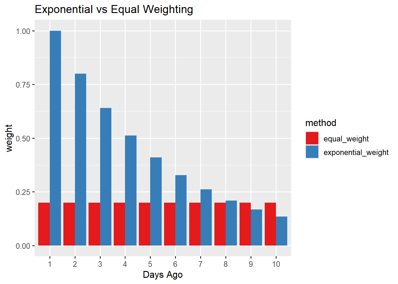
The “exponential” part comes from how the ETS models weight historical data. Unlike a simple moving average where all observations in the window have equal importance, exponential smoothing applies decreasing weights that follow an exponential pattern. Recent points get the highest weight, and the importance decays exponentially as we go further back in time. We demonstrate this in the plot below.
This plot compares how exponential smoothing (80% decay) weights recent data more heavily. It demonstrates how simple averages treat all history equally while exponential smoothing adapts to recent changes. This Makes ETS models particularly responsive to changes in patterns.
15.2 The ETS Framework: Error, Trend and Seasonality
The ETS acronym - which stands for Error, Trend, Season - used for exponential smoothing, reveals the three components these models can incorporate. Each component has different options, resulting in a rich family of models that can adapt to various patterns.
- Error: This tells how randomness affects our predictions. The error could be Additive, which is constant over time or Multiplicative, which is proportional to the level of the series.
- Trend: The long-term direction, This can be None = no trend, Additive = Linear trend or Damped (Ad) = A trend that levels off over time.
- Seasonality: Regular repeating patterns over a fixed period. This can also be None-for no seasonality, Additive - for constant seasonal effect, or Multiplicative - if seasonal effect scales with the level of the series.
A powerful feature of the fable package is its ability to automatically search the space of possible ETS models and select the configuration that best fits the data based on model selection criteria like AIC. We can demonstrate this using our sales training data.
# let fable automatically select the best ETS model
auto_ets <- training_data |>
  model(auto = ETS(Sales))

# examine what model was chosen
report(auto_ets)
Series: Sales
Model: ETS(A,N,N)
Smoothing parameters:
alpha = 0.0001001524
Initial states:
l[0]
28748.26
sigma^2: 101290575
AIC AICc BIC
935.1401 935.7717 940.3531 The ETS() function fits an exponential smoothing model to the data. When no specific component configuration is provided, the function automatically searches for the optimal ETS model for our series. The best model is stored in the auto column of the mable output (auto_ets).We use the report function to display detailed summary of the chosen model, including its final configuration, estimated parameters, and information criteria.
The automatic selection process chose the model ETS(A,N,N). The error is assumed to be Additive, suggesting a constant residual variation over time. No trend and seasonal component were found, the no trend aligns with the visual inspection we have seen in previous chapters however, the no seasonality is a surprising result given the data’s apparent monthly pattern. This means that a SNAIVE benchmark model might still outperform this specific ETS model.
The smoothing parameter \(\alpha\) (alpha) is extremely small (0.0001). This shows that the model almost gives no weight to the most recent observation, relying heavily on the initial level (\(l_0\)) to generate its forecast. Essentially the model defaulted to a MEAN model. Initial states represent the initial level and the value (28748.26) is almost the same as our MEAN model’s estimate from Chapter 14, which is approximately the historical average of the sales data, confirming its mean-based nature.
15.3 Simple Exponential Smoothing
Simple exponential Smoothing (SES) is the most basic form of the ETS framework. It is specifically designed for time series data that exhibits no discernible trend and seasonality. The ETS function requires specifying the components for error (E), trend (T) and seasonality (S) for a particular type of exponential smoothing model. For SES, the trend and seasonality components must be set to None (N).
Smoothing Equation: \(l_t=\alpha\times y_t+(1-\alpha)\times l_{t-1}\)
where: \(l_t\) = the smoothed level at time t, \(y_t\) = the actual observation at time t and \(\alpha\) = the smoothing parameter \((0\le\alpha\le 1)\).
The forecast from this model follows the equation: \(\hat{y}_{t+h}=l_t\), where \(\hat{y}_{t+h}\) is the forecast for \(h\) steps ahead, made at time \(t\) and \(l_t\) is the last calculated smoothed level. In essence, the forecast for all future periods is equal to the most recently smoothed level of the series.
# simple exponential smoothing (level only)
simple_ets <- training_data |>
  model(ses = ETS(Sales ~ error("A") + trend("N") + season("N")))

# Generate forecast
simple_forecast <- simple_ets |>
  forecast(h = 12)

# visualise
simple_forecast |>
  autoplot(training_data) +
  labs(title = "Simple Exponential Smoothing",
       subtitle = "captures only the level - no trend or seasonality",
       y = "Sales", x = "Month")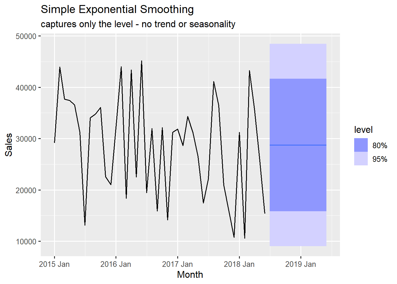
The core function of SES is to track and forecast only the level (or average) of the series, effectively smoothing out random noise while adapting to gradual changes in that average level. ETS(Sales ~ error("A") + trend("N") + season("N")) explicitly defines the components rather than relying on the automatic selection when nothing is specified inside the ETS() function. error("A") specifies an additive error component, trend("N") and season("N") forces the trend and seasonal components to be ignored.
The overall configuration is ETS(A,N,N). Note that this is the same model structure that the automatic selection chose previously. When the forecasts from the model are plotted, they visually confirm its basic function: extending the last calculated average level into the future as seen in Figure 15.2.
Although the SES model only tracks the level of the series, it is essentially a more advanced version of the MEAN model, as it adapts its average based on the most recent data (via the smoothing parameter \(\alpha\)), rather than relying on a fixed historical average. This model would be useful for data like the Ghana Annual GDP Growth Rate, which fluctuates around a constant level ( with no clear trend or seasonality).
15.4 Holt’s Linear Trend Method
The Holt’s linear trend (or Double Exponential Smoothing) model adds trend to capture upward or downward movements. It enhances the simple exponential smoothing model with the addition of a trend component. This makes it ideal to capture information from data showing consistent growth or decline patterns but without seasonality.
We will demonstrate this with the Annual Cereal Yield series from the gh_ts data, which clearly shows an upward trend over time. We first prepare the data by isolating the cereal yield indicator from the rest of the data and performing a train-test split before fitting the model.
# filter gh_ts for the cereal yield
cereal_yield <- gh_ts |>
  filter(indicator_name == "Cereal yield _kg per hectare")

# split data into training and testing
split <- initial_time_split(cereal_yield, prop = 0.75)
training_yield <- training(split)
testing_yield <- testing(split)

# apply Holt's linear trend model
holts_linear <- training_yield |>
  filter(!is.na(value)) |>      # remove missing values to enable ETS fitting
  model(holt = ETS(value ~ error("A") + trend("A") + season("N")))
A 75/30% train-split is performed on the cereal yield series, the model is then fitted on the training series. ETS(value ~ error("A") + trend("A") + season("N")) explicitly forces the model to the additive trend configuration: ETS(A,A,N), with an Additive trend and error and no seasonality. The additive trend is the key component added by Holt’s method. In a double exponential smoothing model, the trend can either be Additive (linear) or Multiplicative (exponential).
15.4.1 Examining the Fitted Model
The Holt’s linear trend method is also called a double exponential smoothing model because it uses two smoothing equations.
- Level Equation: \(l_1=\alpha\times y_t+(1-\alpha)\times(l_{t-1}+b_{t-1})\)
- Trend Equation: \(b_t=\beta\times(l_t-l_{t-1})+(1-\beta)\times b_{t-1}\)
where: \(l_t\) = estimated level at time t, \(b_t\) = estimated trend at time t, \(\alpha\) = level smoothing parameter, \(\beta\) = trend smoothing parameter.
# examine the fitted model
report(holts_linear)
Series: value
Model: ETS(A,A,N)
Smoothing parameters:
alpha = 0.5179828
beta = 0.0001000298
Initial states:
l[0] b[0]
818.8448 9.554271
sigma^2: 11768.84
AIC AICc BIC
627.3173 628.7807 636.5681 The report() function’s output provides insights into the model’s learning process:
- Smoothing Parameter \(\alpha\) (alpha=0.518): This parameter smooths the Level component. A value close to 0.5 means the model gives moderate weight to recent observations, allowing the level to adapt quickly to changes.
- Smoothing Parameter \(\beta\) (beta = 0.0001): This parameter smooths the trend (slope) component. The extremely low value suggest the model found the long term trend (the b[0] initial state) to be very stable and is very slow to adjust the trend based on new data.
- Initial States: The model estimates the starting cereal yield (l[0]) around 819 kg per hectare and the initial growth trend (b[0]) to be approximately 9.55 kg per hectare improvement per year.
15.4.2 Generating and Visualising Forecast
The forecast generation is straightforward using the forecast() function as we have done previously for other models. The Holt’s method follows this equation to calculate the forecast:
Forecast Equation: \(\hat{y}_{t+h}=l_t+h+b_t\), where \(h\) is the forecast horizon.
# generate forecast
holts_forecast <- holts_linear |>
  forecast(h = 5) # 5 year forecast

# visualise forecast with fitted (predicted) values
holts_forecast |>
  autoplot(training_yield) +
  autolayer(holts_linear |> augment(), .fitted, colour = 'red') +
  labs(title = "Holt's Linear Trend",
       subtitle = "Holt's method captures the upward trend in cereal yield")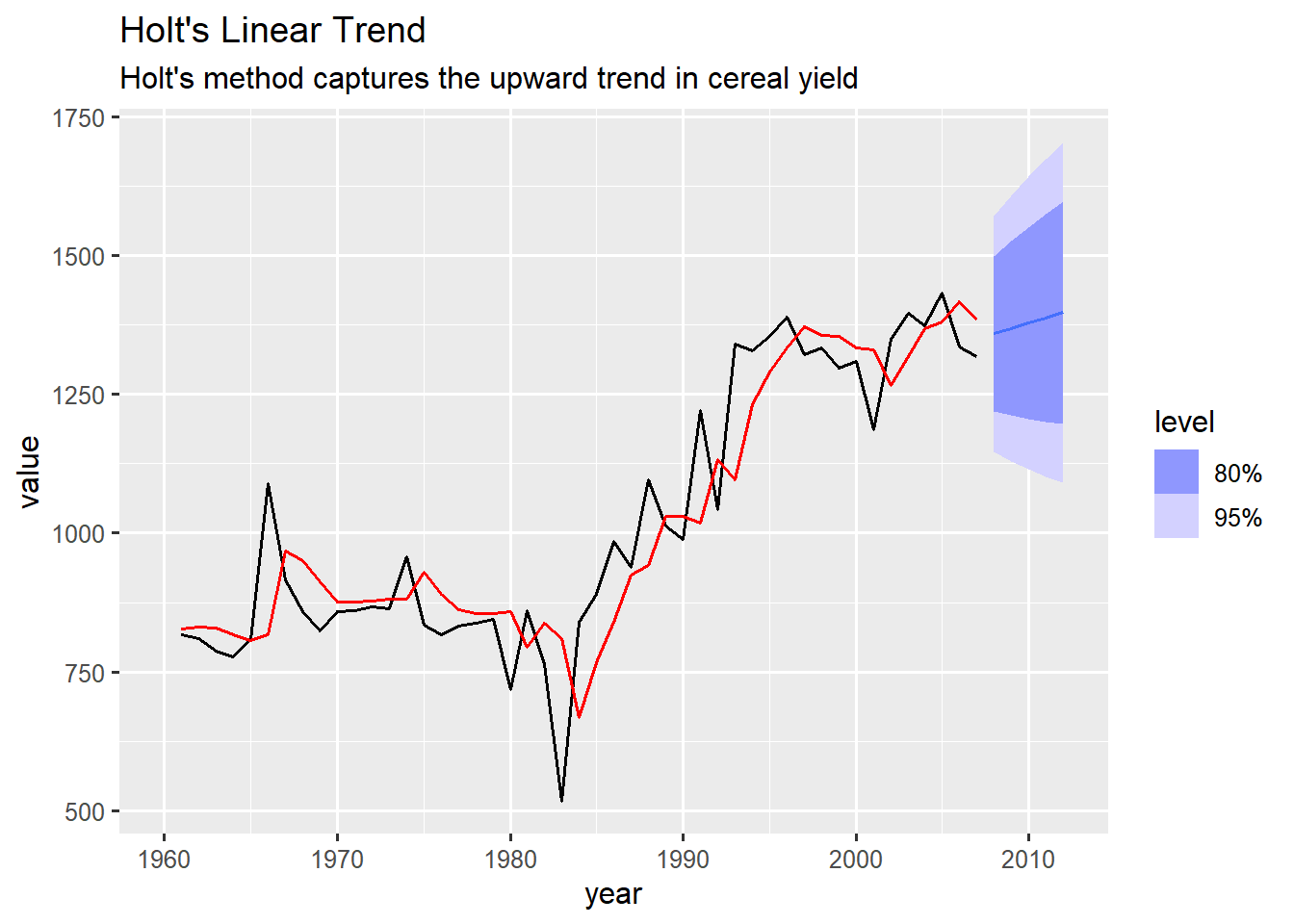
The resulting plot confirms how the models predicted (.fitted) values, the fitted red line, closely tracks the overall upward movement of the cereal yield. This demonstrates that the Holt’s method successfully captures historical trend. The blue forecast line extends linearly into the future, following the rate established by the last smoothed trend. the prediction intervals (shaded area) also widen due to the compounding uncertainty of the trend projection.
This model tracks both the level and linear trend. The trend could be additive (linear) or multiplicative (exponential). This type of model is perfect for series with consistent growth or decline.
15.4.3 Extracting and Visualising Model Components
Another key advantage of the ETS framework is the ability to extract and visualise the underlying components that drive the forecast, using the component() function which we saw in Chapter 10 with the STL decomposition.
# extract and visualise models components
holt_components <- holts_linear |>
  components()

holt_components |> autoplot() +
  labs(title = "Holt's Linear Trend Components",
       subtitle = "Decomposition into level and trend(slope) components",
y = "Cereal Yield") 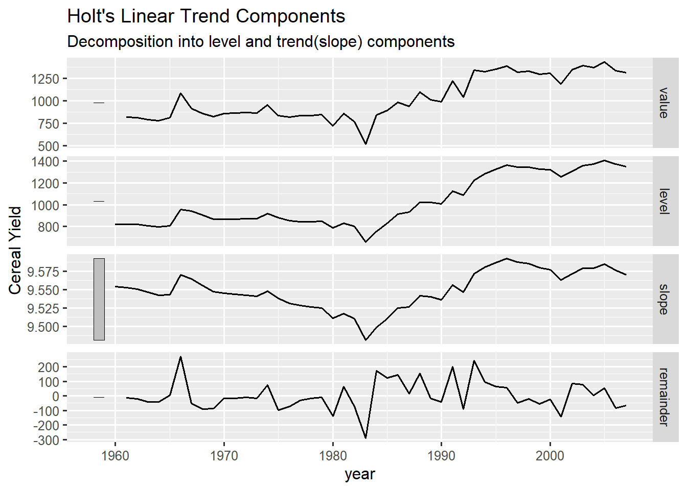
This component plot shows the decomposition of the series in parts that the Holt’s method track. The level shows the smoothed overall level of the series, mirroring the original data’s long-term path but removing noise. The slope shows the smoothed change in the level per year. The plot confirms the slope has been positive for most part of the series though it dips in the early 1980s before rising again. The last part, the remainder, is the residual component. it represents the noise or unpredictable variation left after the level and trend have been accounted for.
Holt’s Linear Trend Method gives us a principled way to forecast series with consistent directional movement, providing a solid middle ground between a simple average and more complex seasonal models.
15.5 Holt-Winters Seasonal Method: The Complete Model
The Holt-Winters Seasonal Method (often referred to as the Holt-Winters method or Seasonal ETS) is the most comprehensive model in the exponential smoothing family. It extends Holt’s linear trend method by adding a dedicated Seasonal component, allowing the model to capture three patterns simultaneously: Level, Trend and Seasonality.
This method is essential for quarterly, monthly, or weekly data that exhibits both long-term growth (or decline) and predictable, recurring fluctuations.
15.5.1 Additive vs. Multiplicative Seasonality
The choice between an additive (A) and multiplicative (M) seasonal component is critical. For an additive seasonality, the seasonal swings are of a constant size regardless of the series’ overall level. This works well when the data is roughly horizontal or the trend is modest. A multiplicative seasonality has seasonal swings that grow in magnitude as the series’ level increases. This is typical for sales or production data that exhibit growth where peaks become higher and troughs become lower over time
We demonstrate the Additive model, ETS(A,A,A), using the quarterly Australian cement production series from the aus_production data, which shows clear seasonality overlaying an upward trend.
# prepare aus_production cement data for model fitting
cement_prod <- aus_production |>
  select(Quarter, Cement)

# split data into training and testing
split <- initial_time_split(cement_prod, prop = 0.75)
training_cement <- training(split)
testing_cement <- testing(split)

# fit a Holt-Winters Seasonal Method (Additive)
hw_additive <- training_cement |>
  model(hw_add = ETS(Cement ~ error("A") + trend("A") + season("A")))
This code for the Holt-Winters model is explicitly configured to track all three components, Level (A), Trend (A) and Seasonality (A).
15.5.2 Examining the Fitted Model
The Holt-Winters method requires three separate smoothing equations (one for each component). Let \(m\) be the length of the seasonality (e.g., \(m=4\) for quarterly data).
- Level Equation: \(l_t=\alpha\times (y_t-s_{t-m})+(1-\alpha)\times (l_{t-1}+b_{t-1})\)
- Trend Equation: \(b_t=\beta\times (l_t-l_{t-1})+(1-\beta)\times b_{t-1}\)
- Seasonal Equation: \(s_t=\gamma\times (y_t-l_{t-1}-b_{t-1})+(1-\gamma)\times s_{t-m}\)
Where \(l_t\) = level: the average value of the series at time t, \(b_t\) = trend: the increasing/decreasing direction of the series at time t and \(s_t\) = the repeating short-term cyclical component at time t. The Equations above are for the Additive variant of the Holt-Winters Method.
# examine fitted model
report(hw_additive)
Series: Cement
Model: ETS(A,A,A)
Smoothing parameters:
alpha = 0.685054
beta = 0.0006119035
gamma = 0.1400382
Initial states:
l[0] b[0] s[0] s[-1] s[-2] s[-3]
522.9393 6.730143 3.348899 58.94868 44.08104 -106.3786
sigma^2: 4690.898
AIC AICc BIC
2217.979 2219.156 2245.823 We see the structure of the model with the specified configuration – the smoothing parameters and initial states with some other relevant information – from the report() output.
Smoothing Parameters: These parameters are responsible for how the model adjusts to each component in the model fitting. The level smoothing parameter (\(\alpha\)) has a relatively high value (0.685), indicating the model gives a strong weight to the most recent observation’s error when updating the level. This means the level adapts quickly to changes in average production. The trend smoothing parameter (\(\beta\)) is extremely low (0.0006), This means the model is very conservative about updating underlying trend (slope) based on new data. It relies heavily on the initial estimate and assumes the long-term growth rate is quite stable. The last smoothing parameter (\(\gamma\)) which is for the seasonality has a moderate value (0.14). This value means the model updates the seasonal factors gradually. It balances the need to reflect recent seasonal performance with the assumption that the quarterly pattern is generally consistent.
Initial States: These are the starting values of components, representing the state of the series before the model began its smoothing process. The initial level (\(l[0]\)) is the estimated baseline production level at the start of the series. The initial trend (\(b[0]\)) is the estimated initial quarterly increase in cement production. The values for \(s[0]\) to \(s[-3]\) represents the initial seasonal factors. They are the initial seasonal effects for each of the four quarters. For instance, s[-1] = 58.95 suggests that Quarter 2 initially saw production about ~59 units above the average level.
15.5.3 Generating and Visualising Forecast
The forecasting operation for the Holt-Winters model takes the final components (\(l_t\), \(b_t\) and \(s_t\)) and projects them into the future \(h\) steps. It is the sum of the last calculated level, trend and seasonal factor, following this equation:
Forecast Equation (Additive): \(\hat{y}_{t+h|t}=l_t+hb_t+s_{t+h-m(k+1)}\)
where \(k\) = the integer or whole number part of \((h-1)/m\) (which ensures we use the most recent seasonal index for the forecast horizon). The forecast() function automatically calculates the this for us.
# generate forecast
hw_forecast <- hw_additive |>
  forecast(h = 12)

# visualise forecast with fitted (predicted) values
hw_forecast |>
  autoplot(training_cement) +
  autolayer(hw_additive |> augment(), .fitted, colour = 'red') +
  labs(title = "Holt-Winters Seasonal Additive Method",
       subtitle = "Holt-Winters method captures the level, upward trend and seasonality")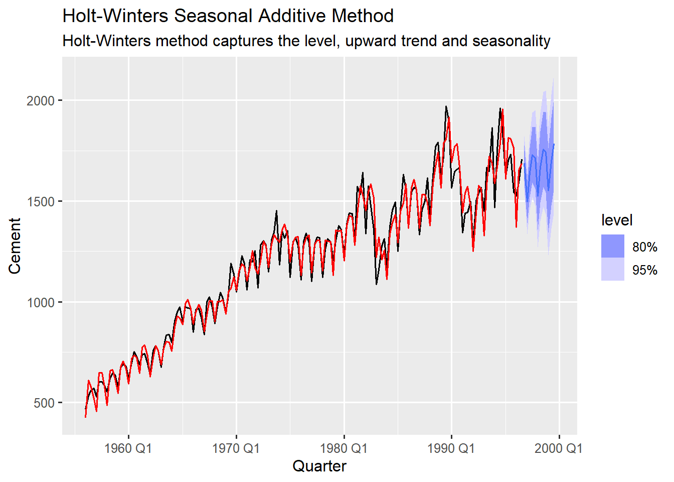
The resulting chart from plotting the original series (black line), the fitted values from the model (red line) and the 12 month forecast (blue line) together shows a powerful visual inspection for validating the models goodness of fit. The red line closely follows the original data, confirming that the smoothing parameters (\(\alpha ,\beta ,\gamma\)) were effectively optimised to track the historical level, trend and seasonality.
The projected blue line in the future exhibits a repeating seasonal pattern overlaid on a linear slightly upward trend, maintaining a constant magnitude for the seasonal peaks and troughs (this is a defining characteristic of the additive model). The prediction intervals (shaded area around forecast) widens as the forecast extends further into the future, reflecting the increasing uncertainty associated with predicting events further ahead in time.
15.5.4 Extracting and Visualising Model Components
The best way to understand what the Holt-Winters ETS model learned from the historical data is through visualisation of the model’s components.
# extract and visualise models components
hw_components <- hw_additive |>
  components()

hw_components |> autoplot() +
  labs(title = "Holt-Winters Seasonal Additive Method's Components",
       subtitle = "Decomposition into level, trend(slope) and seasonal components",
y = "Cement Production") 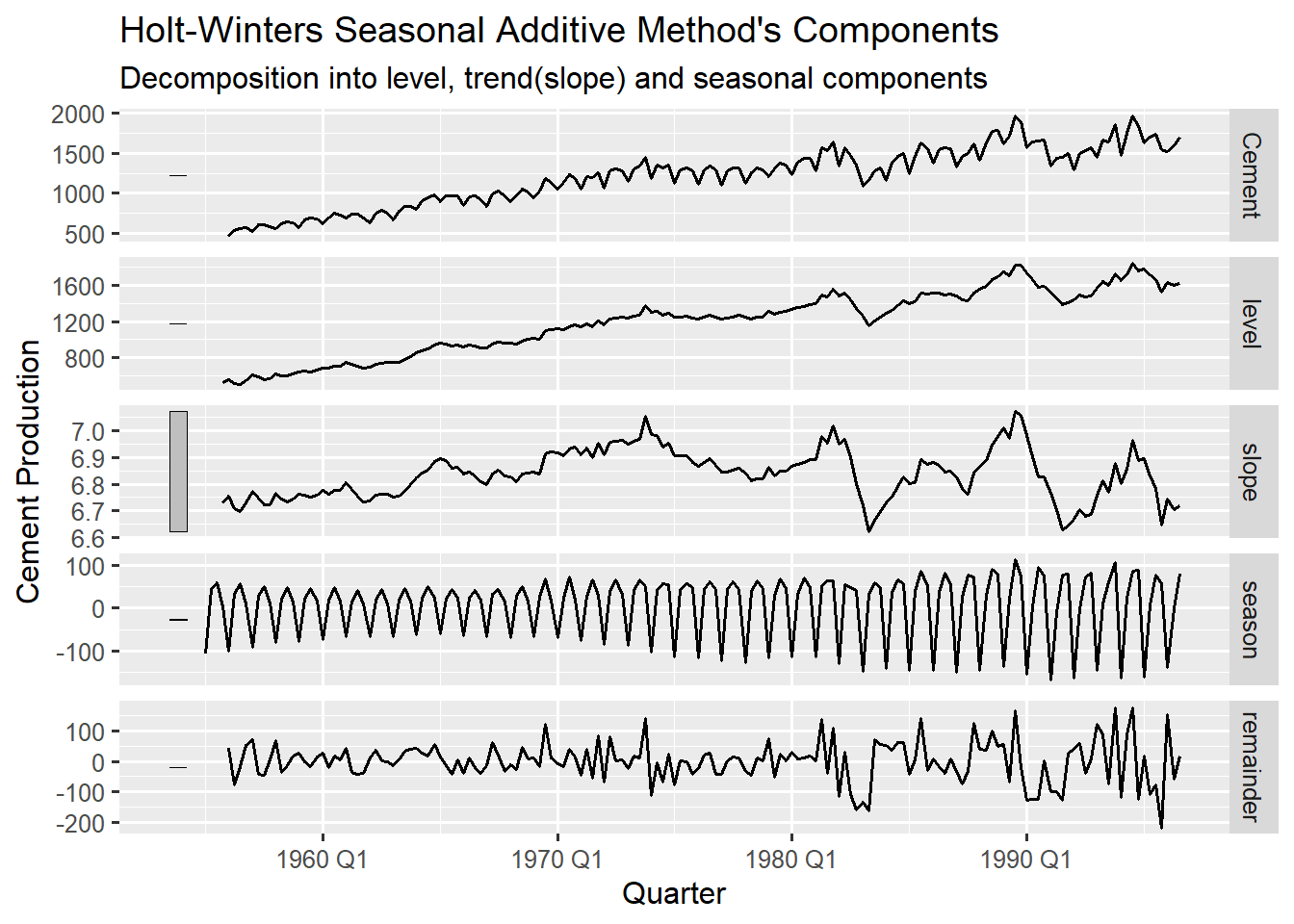
The above figure provides a clear decomposition of the quarterly cement production series. The decomposition contains a plot of the original series, the level, the slope, the seasonal component and the remainder (residuals). The level shows a smooth, long term rising curve that tracks the overall average of the series from the late 1950s through to the early 2000s, removing the short-term noise. This confirms that the average production volume of cement has consistently increased over the long term.
The slope shows the rate of increase per quarter. This component is generally positive and highly smoothed due to the low \(\beta\) value, However the plot reveals the rate of increase was not constant, there are periods where growth accelerated or temporarily slowed. In the early decades (1960s and 1970s) the slope appears positive and relatively stable but experiences significant volatility around 1980s and shows a noticeable decline in the growth rate towards the end of the series (late 1990s). This tells us that, while the production volume continued to rise the pace of that increase may have slowed down or become more erratic.
The seasonal component has a clean, fixed amplitude waveform centred around zero, demonstrating regular quarterly pattern, which is extracted and projected into the forecast. This highly predictable and consistent pattern demonstrates strong quarterly seasonality in the cement production.
The remainder as explained earlier is the residual noise that is left after all three components have been subtracted from the data (unexplained by the model). They appear mostly random suggesting the model has captured the systematic patterns. However there are a few noticeable spikes particularly around the early 1980s and the late 1990s where the model significantly under or over-predicted the actual value.
15.6 Comparing Multiple ETS Models
After understanding the individual ETS components, the logical next step in modelling is to compare several possible configurations to determine which one provides the best representation of the time series dynamics. We use the monthly sales training data (training_data) for this comparison.
# fit multiple ETS configurations
ets_comparison <- training_data |>
  model(
    auto = ETS(Sales),         # let fable decide
    simple = ETS(Sales ~ trend("N") + season("N")),
    holts = ETS(Sales ~ trend("A") + season("N")),
    hw_add = ETS(Sales ~ trend("A") + season("A")),
    hw_mult = ETS(Sales ~ trend("A") + season("M")),
    damped_add = ETS(Sales ~ trend("Ad") + season("A")),  # damped trend (seasonal A)
    damped_mult = ETS(Sales ~ trend("Ad") + season("M"))  # damped trend (seasonal M)
  )
The code above fits 7 different models to to the training_data covering simple, trended, seasonal and damped trend variations. The error components are intentionally left for fable to select, which often defaults to additive (A) but can also choose Multiplicative (M) if it improves fit.
15.6.1 Comparing Training Accuracy (Error Metrics)
Here we will use the accuracy() function to measure how well each model fit the historical data. The models are ranked by MASE, which is the most reliable scale-free metric.
# comparing training accuracy
training_accuracy <- ets_comparison |> accuracy()

training_accuracy |> arrange(MASE)
# A tibble: 7 × 10
.model .type ME RMSE MAE MPE MAPE MASE RMSSE ACF1
<chr> <chr> <dbl> <dbl> <dbl> <dbl> <dbl> <dbl> <dbl> <dbl>
1 hw_mult Training -712. 7554. 5816. -13.2 27.2 0.619 0.630 -0.307
2 damped_mult Training -885. 7726. 6108. -13.9 28.5 0.650 0.644 -0.302
3 damped_add Training -1228. 8011. 6261. -16.0 30.0 0.667 0.668 -0.336
4 hw_add Training -237. 7834. 6360. -11.5 28.9 0.677 0.653 -0.357
5 holts Training 1074. 9747. 8232. -10.7 35.6 0.876 0.812 -0.157
# ℹ 2 more rowsThe Best fit model with lowest MASE is hw_mult (Holt-Winters Multiplicative). The MASE value confirms it has the lowest error compared to a NAIVE benchmark. The Damped Multiplicative and Additive models (damped_mult, damped_add) also show lower MASE error with the additive model showing a slightly higher error than the multiplicative.
Based solely on the training error, the models incorporating a Multiplicative seasonal component (hw_mult and damped_mult) are the best fitting models. This makes intuitive sense for the monthly sales data where peaks and troughs of the seasonal pattern appear to grow proportional to the overall sales level.
15.6.2 Comparing Model Complexity (Information Criteria)
The glance() function extracts information criteria, which penalise model complexity (the number of estimated parameters). The goal is to find the lowest value for AICc (Akaike Information Criterion corrected), as it balances fit and complexity.
glance(ets_comparison) |> arrange(AICc)# A tibble: 7 × 9
.model sigma2 log_lik AIC AICc BIC MSE AMSE MAE
<chr> <dbl> <dbl> <dbl> <dbl> <dbl> <dbl> <dbl> <dbl>
1 auto 101290575. -465. 935. 936. 940. 96467214. 96935527. 8378.
2 simple 101290575. -465. 935. 936. 940. 96467214. 96935527. 8378.
3 holts 105003449. -464. 938. 940. 947. 95003120. 95890263. 8232.
4 hw_mult 0.109 -453. 940. 965. 969. 57061576. 57795032. 0.202
5 hw_add 99146687. -455. 944. 970. 974. 61376521. 62535634. 6360.
# ℹ 2 more rowsThe results from the information criteria reveal a key tension
- The
automodel (which selected ETS(A,N,N)-same as the simple model) has the lowest AIC and AICc - The highly complex
hw_multmodel has a much higher AICc (965.4), despite having a much lower MAE (5816) and MASE (0.619).
This happens because Information Criteria (like AICc) heavily penalise complexity (the number of parameters). The non seasonal ETS(A,N,N) is the simplest, least parameter-intensive (only one smoothing parameter \(\alpha\) and one initial level \(l_0\)) model, so it scores best on complexity, even though it is clearly under-fitting the time series data.
Training accuracy only shows how well a model fits historical noise; information criteria penalise parameters. Neither is a definitive measure of future performance. Given the known seasonality in the sales data, it is highly likely that the simple ETS(A,N,N) model will perform poorly on future unseen data (the testing set). The only way to decide which model will perform better for actual forecast is to conduct cross-validation or, at minimum, evaluate the models on the held-out testing data (more on this in Chapter 17). The hw_mult model which captures the core pattern, is the most likely candidate for the best out of sample performance.
15.7 Generating and Visualising Forecast from Multiple Models
Visualising the forecast from multiple ETS models provides the most intuitive and critical assessment of their behaviour, especially when dealing with contradictory results from accuracy metrics (MASE) and information criteria (AICc).
# generate 12 month forecast from all models
ets_forecasts <- ets_comparison |> forecast(h=12)

# visualise the forecast
ets_forecasts |> autoplot(training_data, level = NULL) +
  scale_colour_brewer(palette = "Set1", type = 'qual')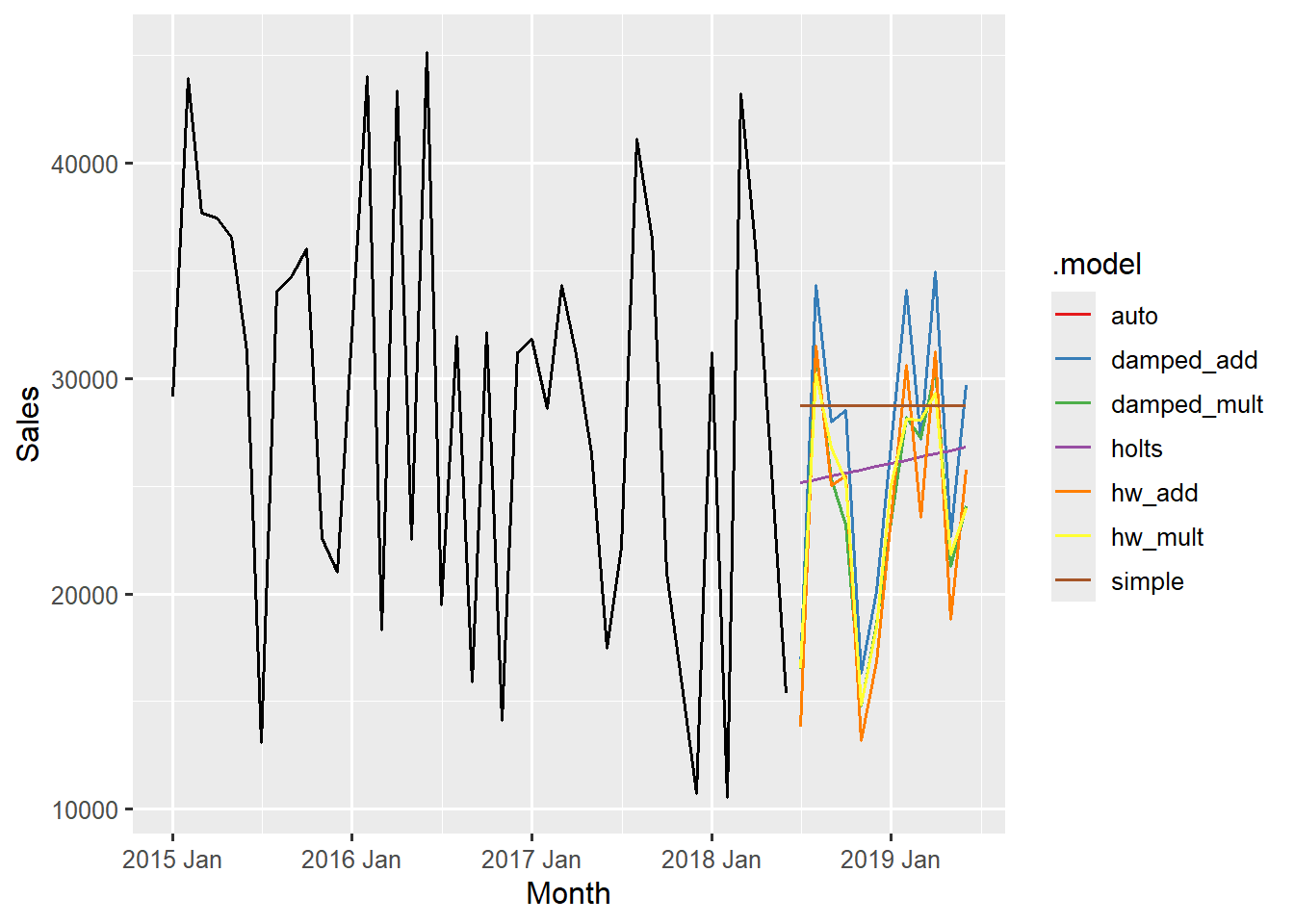
A 12-month forecast is generated for all seven models and plotted against the historical training data. The resulting forecast plot shows distinct behaviours for each model:
Flat-line Models (
auto,simple,holts): The non-seasonal models project flat lines into the future. They fail to capture the monthly seasonality. Thesimpleandautomodels produce the lowest (most conservative) flat forecasts. Theholtsmodel ETS(A,A,N) projects a slightly upward-sloping line, reflecting the minor positive trend it detected, but still missing the cycles.Seasonal Models (
hw_mult,damped_mult,hw_add,damped_add): These models project a cyclical pattern that matches the historical 12-month period. The two best-fitting models from the MASE comparison–Holt-Winters Multiplicative (hw_mult) and Damped Multiplicative (damped_mult), tracks the final period of the training data closely and projects the most reasonable and consistent seasonal cycle forward.
15.7.1 Confirming Historical Goodness of Fit
To validate why the multiplicative models had the lowest training errors, we plot the fitted values (.fitted) against the original series for the top two models: hw_mult and damped_mult.
library(patchwork)

p1 <- training_data |>
  autoplot(Sales) +
  autolayer(ets_comparison |>
              augment() |>
              filter(.model == "hw_mult"), .fitted,
            colour = "red") +
  ggtitle("Holt-Winters Multiplicative Model \nvs Original Series")

p2 <- training_data |>
  autoplot(Sales) +
  autolayer(ets_comparison |>
              augment() |>
              filter(.model == "damped_mult"), .fitted,
            colour = "red") +
  ggtitle("Damped Multiplicative Model \nvs Original Series")

p1+p2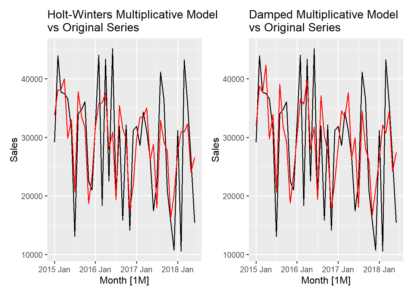
The plot from both models show how extremely well the red fitted line tracks the black original series line, capturing the amplitude of the seasonal peaks and troughs. The superior fit compared to the non-seasonal models confirms that the model’s ability to capture multiplicative seasonality is the primary driver for their low training MAE and MASE values.
The visualisations confirms the initial findings from the error metrics (MASE). Despite having the lowest AICc the simple ETS(A,N,N) model is clearly unsuitable for a highly seasonal series. The Holt-Winters Multiplicative and Damped Multiplicative models offer the most realistic forecasts, making one of them the best choice to evaluate the unseen testing data. The damped_mult model is often preferred in instances like this as its trend component is assumed to level off in the long run, offering a more conservative forecast.
15.8 When to Choose Which ETS Model?
Exponential Smoothing (ETS) models offer a flexible and interpretable framework for time series forecasting. The process of selecting the appropriate ETS model is highly systematic and depends entirely on the patterns (Level, Trend and Seasonality) present in your data.
The ETS framework represented by ETS (Error, Trend, Season), guides model selection using a simple decision tree based on data characteristics.
Does your data have SEASONALITY?
├─ NO → Does it have a TREND?
│   ├─ NO → Use SES: ETS(A,N,N)
│   └─ YES → Does trend flatten?
│       ├─ NO → Use Holt: ETS(A,A,N)
│       └─ YES → Use Damped: ETS(A,Ad,N)
│
└─ YES → What type of seasonality?
    ├─ Constant amplitude → Additive: ETS(A,A,A)
    └─ Growing amplitude → Multiplicative: ETS(M,A,M)
15.8.1 Insights from ETS Modelling in the Fable Framework
The process of fitting and analysing ETS models within frameworks like fable provides valuable lessons applicable to all time series forecasting.
Transparency Builds Trust: Unlike black-box models, you can exactly see how ETS models generate forecasts by extracting and visualising their components.
Damped Trends Often Win: In real-world data forecasting, trends rarely continue indefinitely. Damped trend models often perform best because they realistically assume growth will slow over time.
Multiplicative Seasonality Matters: When your data shows seasonal patterns that grow with the series level (common in business data), multiplicative seasonality provides significantly better fits.
Smoothing Parameters Tell a Story: The \(\alpha\), \(\beta\), and \(\gamma\) values reveal how stable or volatile your series is. High values suggest rapid changes, while low values indicate stable patterns.
Start Simple, Embrace Parsimony: The automatic selection often picks simpler models when they perform nearly as well as complex ones—embracing the principle of parsimony. This reminds us that the best model is the one that captures essential patterns without unnecessary complexity.
15.9 Summary
ETS models give you the perfect blend of sophistication and interpretability. They automatically capture the patterns we identified during exploration while remaining transparent about their reasoning. In our next chapter, we’ll explore ARIMA models — a different but equally powerful approach to time series forecasting.
Remember, the best model isn’t always the most complex one, it is the one that captures the essential patterns in your data while remaining understandable and reliable. ETS models often strike this balance beautifully.