13 Splitting Temporal Data for Modelling
We have now reached a pivotal point in our forecasting journey. Our data has been cleaned, its variance stabilised and stationarity confirmed. Yet, before we proceed to build forecasting models, one fundamental question remains: How will we determine whether our forecasts are truly effective?
This is where proper data splitting becomes essential. Unlike cross-sectional data where random sampling is appropriate, time series data has a strict temporal order that must be preserved. Splitting time series data incorrectly can lead to data leakage, where future information unintentionally influences past predictions, making model evaluations completely unreliable.
13.1 Importance of Temporal Splitting
In standard predictive models that uses cross-sectional data like linear regression, the goal is to predict an outcome without regard to order, so random train-test splitting is common. However, with time series data care must be taken to maintain the chronological order when splitting because it has observations that are dependent on previous observations (autocorrelation).
A random split ignores the time dependency, leading to data leakage and unrealistic evaluations. First, we need to understand why time series requires special care when splitting.
The above code creates a random 70/30 split. We set a seed ‘set.seed(523)’ so that the random numbers generated will remain the same any time the code runs. This approach is problematic because the testing points are scattered throughout the timeline as displayed in Figure 13.1 below. Fitting a model using this data could make it appear accurate by “memorising” nearby values, but will fail in real forecasting scenarios.
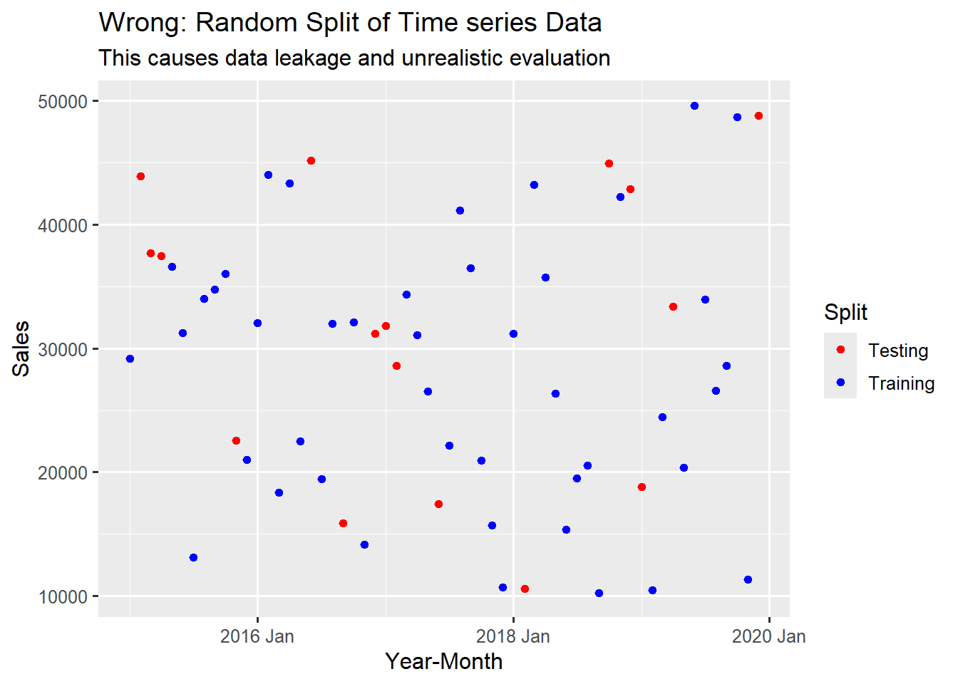
This plot shows a clear example of data leakage because the model will train on past data but then has to predict values for periods where it has already seen future information (e.g., training on 2019 sales but testing on 2016 sales).
A model evaluated this way will report optimistically high accuracy on the test data because it is not performing true forecasting into an unknown future (unrealistic evaluation).
13.2 Proper Temporal Train-Test Splitting
The correct approach is to maintain the temporal order, using earlier data for training and later data for testing. When this happens, the model uses the past to predict the future which is exactly what we need our model to do.
# proper temporal split
temporal_split <- sales_ts |>
  mutate(
    Split = if_else(Month < yearmonth("2018 Jul"), "Training", "Testing")
  )
This new code splits the data based on a specific time point. All data before July 2018 is used for training and all data after for testing. This preserves the temporal sequence as can be seen in Figure 13.2 below, and simulates real forecasting scenarios.
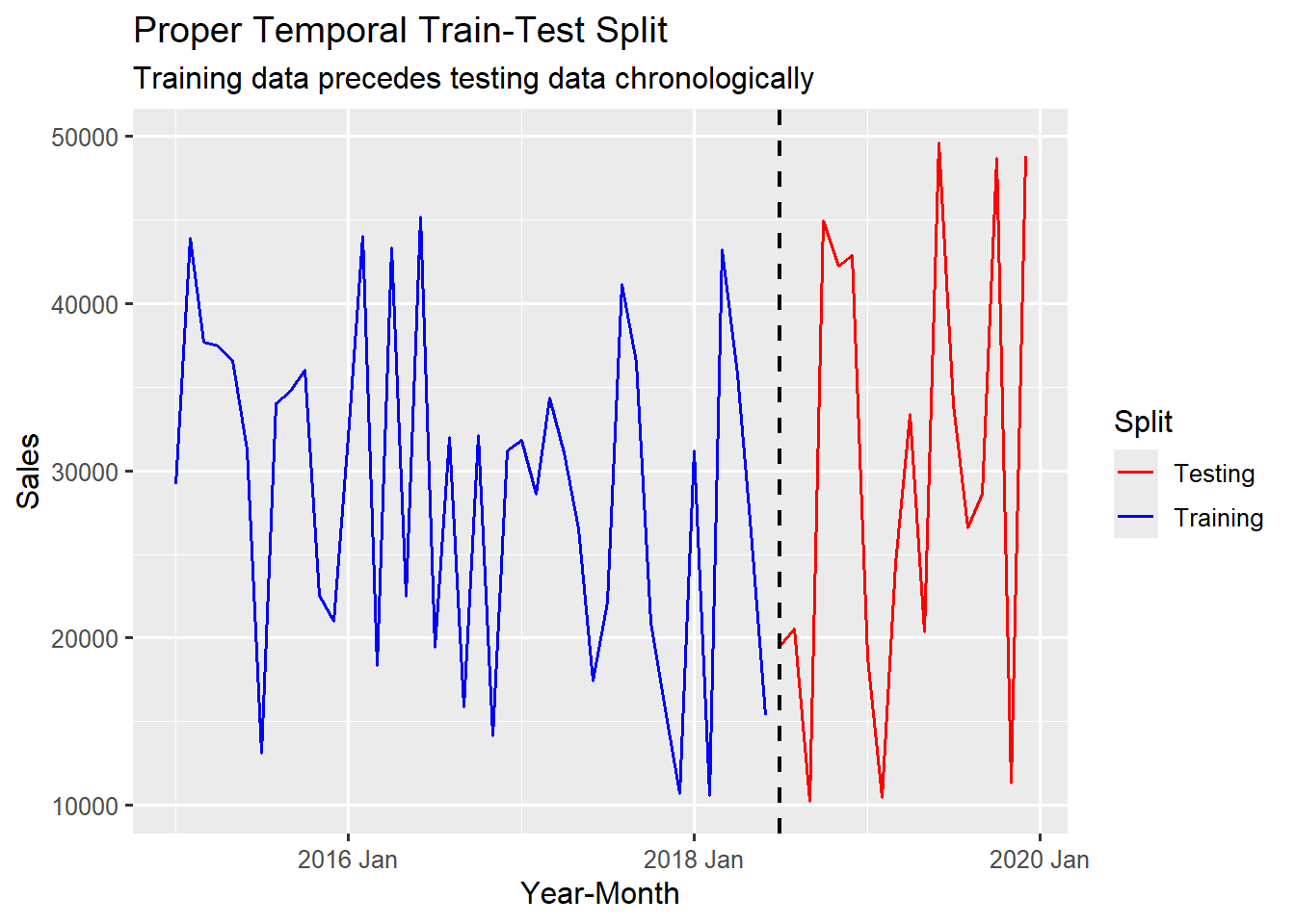
We see in this plot how the entire data before the split point (dashed vertical line - July 2018) is used as the training data (blue), followed orderly by the testing data (red). This train-test split is necessary for a valid forecasting evaluation.
13.2.1 Creating Training and Testing Datasets
Now we can formally create our training and testing datasets the right way. To make the splitting easier, we are going to use the initial_time_split() function from the rsample package. This function will automatically split the data proportionally while maintaining the temporal order.
# create formal training and testing datasets
library(rsample)

split <- initial_time_split(sales_ts, prop = 0.7)

training_data <- training(split)
testing_data <- testing(split)

# verify order of splits
partition_table <- tibble(
  Partition = c("training data", "testing data"),
  Start_period = c(min(training_data$Month),
                   min(testing_data$Month)),
  End_period = c(max(training_data$Month),
                 max(testing_data$Month)),
  N_Obs = c(nrow(training_data), nrow(testing_data))
)| Partition | Start_period | End_period | N_Obs |
|---|---|---|---|
| training data | 2015 Jan | 2018 Jun | 42 |
| testing data | 2018 Jul | 2019 Dec | 18 |
initial_time_split(sales_ts, prop = 0.7) is the core function for our temporal splitting. It takes our time series data (sales_ts) and automatically creates the split object such that the first \(70\%\) (prop = 0.7) of the data chronologically forms the training set, and the remaining \(30\%\) forms the testing set.
training(split) / testing(split) are accessor functions that extract the actual data frames (tibble) for the respective partitions. To confirm we have the right train-test split, we create a table to verify the chronological order. As expected we see in the table that the test data is immediately after the end date of the training data, confirming that the split is purely temporal and not random.
13.3 Time Series Cross-Validation
For more robust model evaluation, we can use time series cross-validation (TSCV). This creates multiple training and testing folds while preserving temporal order. We use the stretch _tsibble() function from the tsibble package to create cross-validation (cv) folds in a time series data.
# create time series cross-validation folds
tscv_folds <- training_data |>
  stretch_tsibble(.init = 26, .step = 1)

# examine the cross-validation structure
cv_summary <- tscv_folds |>
  as_tibble() |>
  group_by(.id) |>
  summarise(
    start_date = min(Month),
    end_date = max(Month),
    n_obs = n(),
    .groups = "drop"
)| .id | start_date | end_date | n_obs |
|---|---|---|---|
| 1 | 2015 Jan | 2017 Feb | 26 |
| 2 | 2015 Jan | 2017 Mar | 27 |
| 3 | 2015 Jan | 2017 Apr | 28 |
| 4 | 2015 Jan | 2017 May | 29 |
| 5 | 2015 Jan | 2017 Jun | 30 |
| 6 | 2015 Jan | 2017 Jul | 31 |
| 7 | 2015 Jan | 2017 Aug | 32 |
| 8 | 2015 Jan | 2017 Sep | 33 |
| 9 | 2015 Jan | 2017 Oct | 34 |
| 10 | 2015 Jan | 2017 Nov | 35 |
| 11 | 2015 Jan | 2017 Dec | 36 |
| 12 | 2015 Jan | 2018 Jan | 37 |
| 13 | 2015 Jan | 2018 Feb | 38 |
| 14 | 2015 Jan | 2018 Mar | 39 |
| 15 | 2015 Jan | 2018 Apr | 40 |
| 16 | 2015 Jan | 2018 May | 41 |
| 17 | 2015 Jan | 2018 Jun | 42 |
stretch_tsibble(.init = 25, .step = 1) creates expanding window folds. .init sets the initial training window size and .step specifies how many months to move forward for each fold. Our code creates multiple folds where each fold starts with at least 25 observations (months) and expands by 1 observation each time. Here the first fold uses months 1 to 25 for training and month 26 for testing. The next fold uses months 1 to 26 for training and month 27 for testing and so on till the end of the series.
Each fold is marked by an .id column allowing us to track different train-test combinations. This approach provides multiple evaluations across different time periods.
13.3.1 Visualise Cross-Validation Folds
Let’s visualise how our cross-validation works.
# visualise the first few cross-validation folds
tscv_folds |>
  filter(.id <= 4) |>      # show first 4 folds
  group_by(.id) |>         # temporarily group data
  mutate(
    fold_info = paste("Fold",.id,": ",first(Month)," to ",last(Month)),
  ) |>
  ungroup() |>             # remove grouping
  ggplot(aes(x = Month, y = Sales, group = .id)) +
  geom_line(linewidth = 0.7) +
facet_wrap(vars(fold_info), ncol = 2) 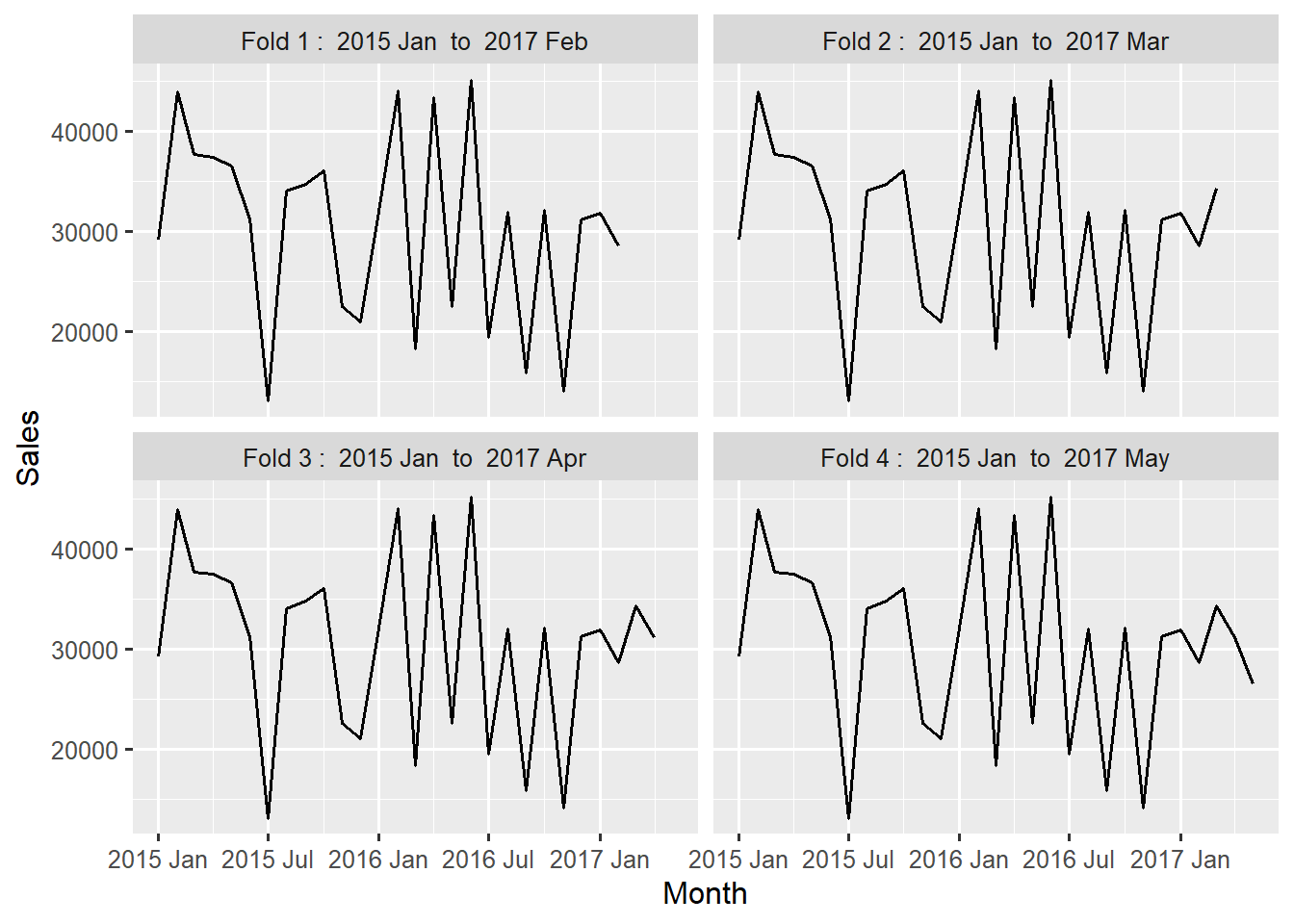
The above plot displays the expanding nature of the cross-validation folds produced from stretch_tsibble(). We clearly see how each fold contains all the data from the previous fold plus the additional (step) month.
13.3.2 Rolling Window Analysis
Another way to create cv-folds is by using the slide_tsibble() function. This function differs slightly from stretch_tsibble() in the way they generate folds. slide_tsibble() creates overlapping windows of data that move step by step.
# implement walk forward validation
walkf_cv_folds <- training_data |>
  slide_tsibble(.size = 28, .step = 1)

# examine the walk-forward cv structure
walkf_cv_summary <- walkf_cv_folds |>
  as_tibble() |>
  group_by(.id) |>
  summarise(
    start_date = min(Month),
    end_date = max(Month),
    n_obs = n(),
    .groups = "drop"
)| .id | start_date | end_date | n_obs |
|---|---|---|---|
| 1 | 2015 Jan | 2017 Apr | 28 |
| 2 | 2015 Feb | 2017 May | 28 |
| 3 | 2015 Mar | 2017 Jun | 28 |
| 4 | 2015 Apr | 2017 Jul | 28 |
| 5 | 2015 May | 2017 Aug | 28 |
| 6 | 2015 Jun | 2017 Sep | 28 |
| 7 | 2015 Jul | 2017 Oct | 28 |
| 8 | 2015 Aug | 2017 Nov | 28 |
| 9 | 2015 Sep | 2017 Dec | 28 |
| 10 | 2015 Oct | 2018 Jan | 28 |
| 11 | 2015 Nov | 2018 Feb | 28 |
| 12 | 2015 Dec | 2018 Mar | 28 |
| 13 | 2016 Jan | 2018 Apr | 28 |
| 14 | 2016 Feb | 2018 May | 28 |
| 15 | 2016 Mar | 2018 Jun | 28 |
slide_tsibble(.size = 28, .step = 1) creates fixed-size windows that slides forward. Here size = 28 uses 28 months for the first fold (fixed) and each new fold (window) moves forward by 1 month (.step = 1).
The key difference between the stretch_tsibble() and slide_tsibble() functions is that the former uses expanding folds (i.e., training sets grow over time) whiles the latter uses fixed folds (old observations drop off as new ones come in, keeping the window fixed). Implementing TS-CV either with stretch_tsibble or slide_tsibble provide more robust model error estimates than a single train-test split.
13.4 Handling Multiple Series’
When dealing with a collection of time series (tsibble with 2 or more keys), a proper train-test split must be applied to each series individually but based on a consistent temporal rule.
13.4.1 Consistent Temporal Splitting by Date
This demonstration manually applies a split boundary (year < 2005) to a selection of indicator names in the gh_ts tibble.
# split multiple series consistently
multi_series_split <- gh_ts |>
  filter(indicator_name %in% c(
    "Annual GDP growth rate",
    "Cereal yield _kg per hectare",
    "Gross national expenditure (% of GDP)"
  )) |>
  select(indicator_name, year, value) |>
  group_by(indicator_name) |>
  mutate(
    split = if_else(year < 2005, "Training", "Testing")
    ) |>
  ungroup()
In order to apply the split boundary logic to all the series independently, the data is grouped by their unique indicator name. The consistent temporal rule specified in the mutate function creates a marker for the training and testing split.
All data before the year 2005 \((~70%)\) is marked as the training set and 2005 upwards \((~30)\) is the testing set.
# visualise the splits for all series
multi_series_split |>
  ggplot(aes(x = year, y = value, colour = split)) +
  geom_line(linewidth  = 0.7) +
  facet_wrap(vars(indicator_name), scales = "free_y", ncol = 2) +
  scale_colour_manual(values = c("red", "blue")) +
  theme(legend.position = "bottom")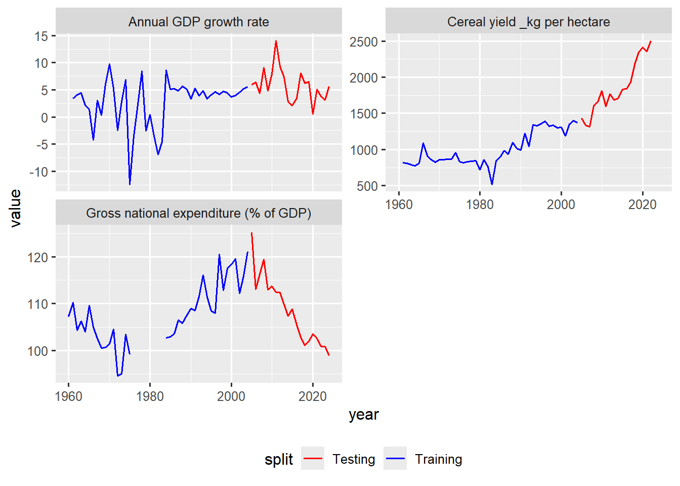
Visualising the series, we see that each of the three indicators - GDP growth rate, Cereal yield and GNE (% of GDP) - are all split exactly at the year 2005, as indicated by the separate red and blue lines. This confirms our intended chronological split for each series where the training period precedes the testing period for all series simultaneously.
13.4.2 Automated Splitting and Extraction
While manual splitting works, automatically creating and extracting the training and testing datasets for many series requires a more programmatic approach compared to doing the same for a single series by utilising some useful functions from the purrr and rsample packages.
A. Applying the Split per Series Key
The fable ecosystem relies on the key columns (here, indicator_name) to perform operations across multiple series in a tsibble.
# apply initial time split per key
splits_multiple <- gh_ts |>
  filter(indicator_name %in% c(
    "Annual GDP growth rate",
    "Cereal yield _kg per hectare",
    "Gross national expenditure (% of GDP)"
  )) |>
  select(indicator_name, year, value) |>
  group_by_key() |>
  group_map(~ initial_time_split(.x, prop = 0.7))
The group_by_key() function is specific to tsibbles. It groups the data by the unique time series identifier (indicator_name). The core operation of what we want to achieve is carried out by the group_map() function, which iterates over each series (each indicator) and applies the initial_time_split() function to create a chronological split, using the first \(70\%\) of the observations for training. The resulting output from this code is a list of 3 split objects, each representing a unique series.
[[1]]
<Training/Testing/Total>
<45/20/65>

[[2]]
<Training/Testing/Total>
<45/20/65>

[[3]]
<Training/Testing/Total>
<45/20/65>
B. Extracting and Organising the Datasets
This next code uses purrr’s map() function to extract the training and testing datasets from the list of split objects, and then organising them into a tidy tibble.
# extract training and testing sets and convert back to tsibble
train_sets <- map(splits_multiple, training) |>
  lapply(as_tsibble, index = year)

test_sets <- map(splits_multiple, testing) |>
  lapply(as_tsibble, index = year)

# combine with labels (indicator names) and convert to a tidy tibble
keys <- gh_ts |>
  filter(indicator_name %in% c(
    "Annual GDP growth rate",
    "Cereal yield _kg per hectare",
    "Gross national expenditure (% of GDP)"
  )) |>
  distinct(indicator_name) |> pull()

multi_split_list <- tibble(
  series = keys, training = train_sets, testing = test_sets
)
the map() function works similarly to the group_map() function. It also iterates through the list of split objects (splits_multiple) and applies the training() and testing() accessor functions to each one , returning a list of three separate training and testing tibbles (one for each series). The lapply() function converts all the returned tibbles back to time series tsibbles.
We then combine everything into a single structured tibble (multi_split_list)
# A tibble: 3 × 3
  series                                training          testing
  <chr>                                 <list>            <list>
1 Annual GDP growth rate                <tbl_ts [45 × 2]> <tbl_ts [20 × 2]>
2 Cereal yield _kg per hectare          <tbl_ts [45 × 2]> <tbl_ts [20 × 2]>
3 Gross national expenditure (% of GDP) <tbl_ts [45 × 2]> <tbl_ts [20 × 2]>
The multi_split_list object is a tidy summary where each row represents a single time series, and the training and testing columns contain the properly split tsibbles. This structure is ideal for cross-validation and concurrent model fitting on multiple series.
13.5 Summary
In this chapter we have addressed an important aspect of time series forecasting; creating a validation framework that produces honest, reliable performance assessments. We moved beyond simple random sampling to embrace the temporal nature of our data.
You have seen the reason why preserving chronological order prevents data leakage and ensures realistic model evaluation. You now understand that testing should always follow training in time and performing cross-validation on time series gives us multiple assessments of model performance, making our evaluation more reliable than a single train-test split.
With our data properly prepared, variance stabilised, stationarity achieved and rigorous validation splits established we are now ready for the most exciting phase: building actual forecasting models. In our next section we will explore various forecasting models and how they effectively fit to our temporal data.