# load and prepare cocoa price data
cocoa_ts <- gh_cocoa |>
  mutate(Date = yearmonth(Month)
         ) |>
  as_tsibble(index = Date) |>
  select(Date, Price)

# split into training and testing set (use 75% for training and 25% for testing)
split <- initial_time_split(cocoa_ts, prop = 0.75)
training_cocoa <- training(split)
testing_cocoa <- testing(split)17 Model Evaluation and Forecasting
We have now reached the final and important stage of our time series journey where we bring everything together. After cleaning and preparing our data, exploring patterns and building both simple and advanced forecasting models, we now face the ultimate test; determining which models actually work in practice and deploying them responsibly. Think of this chapter as your forecasting graduation ceremony.
This chapter is not just about technical metrics – it is developing judgement to separate reliable forecast from wishful thinking. We will learn how to compare models objectively, understand their uncertainties, and create production-ready forecasting systems that deliver real value whether you are predicting sales, weather, yeild or website traffic.
17.1 Fitting Multiple Models and Generating Forecasts
In the real world, relying on a single forecasting model is like bringing only one tool to a construction site. Imagine you are investing in stocks. Would you put all your money in a single company? Ofcourse not! You would diversify. No single model is perfect for all situations so smart forecasters create a model portfolio. Building different models help to capture different aspects of your data, and by creating a diverse model portfolio, you gain both robustness and insights.
17.1.1 Data Preparation: Cocoa Prices
We introduce a new dataset (gh_cocoa.csv) for this work. This data was obtained from the Bank of Ghana website (https://www.bog.gov.gh/economic-data/commodity-prices/), and it contains the average monthly Cocoa Prices in USD per Tonne from January 2000 to April 1 2023.
SInce cocoa prices are notoriously volatile, influenced by weather, global demand, and economic policies, they make an ideal candidate for a multi-model approach.
First we load and prepare the raw data into a tsibble format suitable for time series analysis and then create a temporal split with the initial_time_split() function. We use 75% of the data (Jan 2020 - roughly mid 2017) for training and the remaining 25% (roughly mid 2017 - April 2023) for testing.
17.1.2 Building a Comprehensive Model Portfolio
We use the fable workflow to simultaneously fit a wide range of models to the training data. Each model represents a different hypothesis about how the cocoa prices evolve.
# build comprehensive model portfolio
cocoa_model_portfolio <- training_cocoa |>
  model(
    # Benchmark models
    naive = NAIVE(Price),
    seasonal_naive = SNAIVE(Price),
    mean = MEAN(Price),

    # Exponential Smoothing Family
    ets_auto = ETS(Price),
    ets_hw_mult = ETS(Price ~ trend("A") + season("M")),
    ets_damped = ETS(Price ~ trend("Ad")),

    # ARIMA family
    arima_auto = ARIMA(Price),
    arima_log = ARIMA(log(Price)),
    arima_seasonal = ARIMA(log(Price) ~ pdq(0,1,1) + PDQ(0,0,1)),

    # Other simple linear models
    linear = TSLM(Price ~ trend()),
    linear_season = TSLM(Price ~ trend() + season())
  )
Eleven different models are created in our portfolio of models spanning simple benchmark models to sophisticated approaches.
Benchmark Models
-
naiveassumes the future price will be exactly the same as the last observed price (random walk). -
seasonal_naiveassumes the price next January will be the same as last January. -
meanpredicts the historical average price.
Exponential Smoothing (ETS) Family
-
ets_autolets the algorithm automatically select the best combination of error, trend and seasonality based on AICc. -
ets_hw_mult(Holt-Winters Multiplicative), explicitly models a linear trend and seasonality that grows in magnitude as prices rise. -
ets_dampedmodels a trend that eventually flattens out (damped), assuming price rallies or crashes will not last forever.
ARIMA Family
-
arima_autoautomatically selects the best orders \((p,d,q)(P,D,Q)\) to handle correlations and stationarity -
arima_logfits an ARIMA model to the the log transformed prices; this stabilises variance. -
arima_seasonal: explicitly forces the model to use the specified non-seasonal and seasonal autoregressive and moving average orders.
Linear Models
-
linearfits a simple straight line (regression) through the data; assuming a constant rate of price increase/decrease over time. -
linear_seasonfits a straight line but adds a fixed “dummy” effect for each month assuming a constant additive seasonality.
This ensemble of models create a powerful “tournament” where we can rigorously test which mathematical description best matches the reality of the cocoa market.
17.1.3 Generating a 2-Year forecast
With our diverse portfolio of models fitted to the historical data, we can now project the behaviour of cocoa prices into the future. This is the moment where each model applies its learned patterns – trend, seasonality, and level – to predict what comes next.
We will generate a 24-month (2-year) forecast for all models in our portfolio.
# generate 24 month forecast from all models
cocoa_forecasts <- cocoa_model_portfolio |>
  forecast(h = 24)

# view forecasts
cocoa_forecasts |> hilo()
# A tsibble: 264 x 6 [1M]
# Key: .model [11]
.model Date
<chr> <mth>
1 naive 2017 Jul
2 naive 2017 Aug
3 naive 2017 Sep
4 naive 2017 Oct
5 naive 2017 Nov
# ℹ 259 more rows
# ℹ 4 more variables: Price <dist>, .mean <dbl>, `80%` <hilo>, `95%` <hilo>The forecast produces a probabilistic prediction for each model for every future month including 80% and 95% confidence intervals. By comparing the forecasts from each model, we can gauge the consensus or divergence in the market outlook.
17.2 Visualising and Comparing Forecasts
A well crafted visualisation can reveal more than a table of metrics. Let’s see all our forecasts with the historical data. This helps to reveal consensus, divergence and model uncertainties far more effectively than reading a table of numbers. Since the models in the portfolio operate under different mathematical assumptions, their projections for the future will vary significantly.
17.2.1 Portfolio Forecast Plot (Consensus & Divergence)
# plot all forecasts against historical data
cocoa_forecasts |>
  autoplot(training_cocoa, level = 95) +
  labs(title = "Ghana Cocoa Prices: 24-Month Forecasts from 11 Models",
       subtitle = "shaded areas show 95% prediction intervals")+
  scale_y_continuous(labels = scales::dollar_format()) +
  theme(legend.position = "none")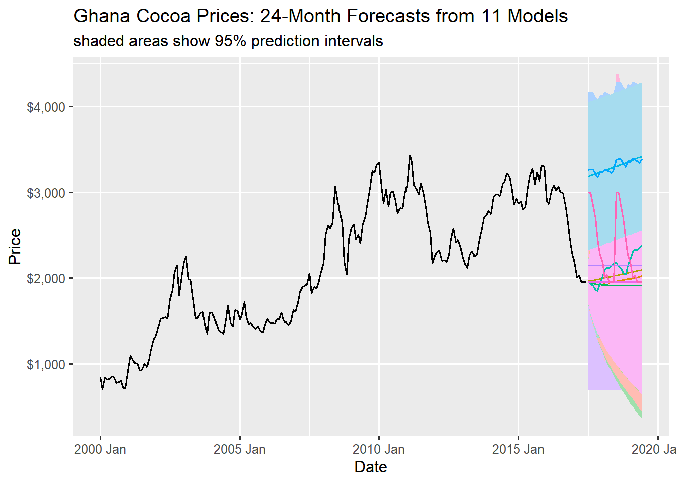
The plot in Figure 17.1 overlays all 11 forecasts onto the historical price series, highlighting the end of the training data (mid-2017) and the 24-month forecast period. The 11 models show high divergence. The forecast lines cluster tightly near the start of the forecast horizon but diverge dramatically over the 24 months. The blue, orange, and pink shaded areas cover a huge vertical span, indicating extremely high uncertainty about the cocoa prices.
Many models (the \(\text{ETS}\) and \(\text{ARIMA}\) models) predict that the price will remain relatively flat or slightly trend upward from the starting point of approximately \(\$2,000\) to \(\$2,500\). The seasonal naive (SNAIVE) model (optimistic model) predicts a strong cyclical rebound, taking prices to over \(\$3,000\) by the end of the horizon.
In summary, clustered lines suggest models agree, while diverging or large separated lines suggest high prediction uncertainty between models. Analysts must treat this forecast with caution as the 95% interval spans thousands of dollars.
17.2.2 Individual Model Forecasts
For a cleaner presentation you would want a clear visualisation of each model’s forecast in a different panel.
# create separate panels for each model
cocoa_forecasts |>
  autoplot(training_cocoa, level = 95) +
  facet_wrap(~.model, nrow = 4) +
  theme(legend.position = "none") +
  scale_y_continuous(labels = scales::label_currency()) +
  scale_x_yearmonth(date_breaks = "5 years") +
  labs(title = "Individual Model Forecasts for Ghana Cocoa Prices",
       subtitle = "Training period: 2000-2017 | Forecast horizon: 24 months")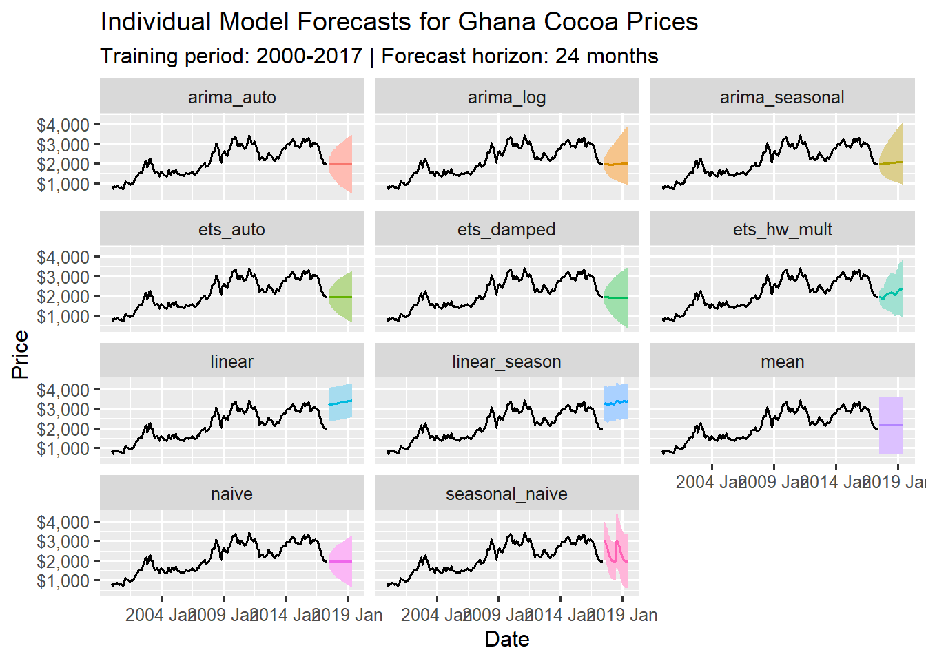
Figure 17.2 presents each model’s forecast in a separate panel for easy identification and interpretation. The mean, naive and ets_auto models projects flat lines into the future.The arima_seasonal and ets_hw_mult captures some seasonality with a mild upward drift. The linear models show a consistent upward trend with the linear_season accounting for some seasonality using seasonal dummy variables. The seasonal_naive shows a strong highly volatile seasonal cycle, projecting massive price swings based on the last years pattern.
The overall comparison emphasizes the need for Model Evaluation on unseen data, as the choice between conservative stability and aggressive volatility in some models is still unresolved.
17.3 Model Accuracy Assessment Framework
A good forecast is not just about low errors , it is about getting close to the actual values. Accuracy metrics tell us how wrong our models are, but different metrics emphasise different errors. Understanding these nuances is crucial for selecting the right model for your specific use case.
17.3.1 Initial Evaluation on Training Data
We begin by assessing the models’ performance on the training data – the historical period used to fit the model parameters. This shows how well each model captures the known historical patterns.
# calculate model accuracy on training data
training_accuracy <- cocoa_model_portfolio |>
  accuracy() |> select(.model, MASE, RMSE, MAPE, MAE)

training_accuracy |> arrange(MASE)
# A tibble: 11 × 5
.model MASE RMSE MAPE MAE
<chr> <dbl> <dbl> <dbl> <dbl>
1 arima_seasonal 0.265 134. 5.02 102.
2 arima_auto 0.265 134. 5.03 102.
3 arima_log 0.267 134. 5.00 103.
4 ets_damped 0.268 136. 5.07 103.
5 ets_auto 0.269 136. 5.08 104.
# ℹ 6 more rowsThe ARIMA/ETS models form the top 5 best performing models with \(MASE \approx 0.26\). The seasonal_naive model is the baseline error for the seasonal cycle (\(MASE = 1\)). The non-seasonal naive (naive) model has an \(MASE\) of \(0.27\). The fact that it is much better than the seasonal naive model suggests that the cocoa prices lack a stable repeating monthly seasonal pattern.
The linear models perform poorly (\(MASE \approx 0.88\)) compared to the others, indicating that simple regression fails to capture the high volatility and non-linear trend of the cocoa prices.
Interpreting Key Accuracy Metrics
| Metric | What It Measures | Example Interpretation | Good for Cocoa Prices? |
|---|---|---|---|
| MAE | Average dollar error | “We are usually off by $100/tonne” | Yes – easy to understand |
| RMSE | Square root average squared error | “Big mistakes hurt us badly” | Yes – penalises large errors |
| MAPE | Percentage error | “We are usually off by 12%” | Yes – comparable across time |
| MASE | Error vs naive forecast | 0.8 = 20% better than naive (baseline) | Yes – best overall metric |
A common pitfall is relying solely on point forecast metrics like RMSE or MAE. A model with great RMSE but terrible interval coverage is unreliable for risk management. After selecting the best model based on MASE, it is crucial to check the accuracy on the held out test data and verify the interval coverage. But before selecting the best model and validating on the test data we will perform a time series cross validation.
17.4 Time Series Cross Validation and Model Selection
Traditional train-test splits can be misleading for time series because they only evaluate performance at one specific historical cut-off. . Time series cross-validation (TSCV) provides a more robust and realistic assessment by testing models on multiple historical periods. This simulates many “what if?” scenarios over the series’ lifetime, leading to a more reliable error estimate.
17.4.1 Implementing Time Series Cross-Validation
We use the expanding window approach (stretch_tsibble()) to create sequential training folds from the training data. Chapter 13 explains in detail how to create time series cross-validation folds.
# create time series cross validation
cocoa_cv <- training_cocoa |>
  stretch_tsibble(.init = 120, # 10-year initial fold
                  .step = 6    # roll forward 6 months
                )
The core of the TSCV process is fitting the model portfolio to every single fold and then calculating two things; the fit quality (using \(AICc\)) and the out-of-sample accuracy (\(MASE\)).
# perform rolling origin evaluation
cv_models <- cocoa_cv |>
  model(
    naive = NAIVE(Price),
    seasonal_naive = SNAIVE(Price),
    mean = MEAN(Price),
    ets_auto = ETS(Price),
    ets_hw_mult = ETS(Price ~ trend("A") + season("M")),
    ets_damped = ETS(Price ~ trend("Ad")),
    arima_auto = ARIMA(Price),
    arima_log = ARIMA(log(Price)),
    arima_seasonal = ARIMA(log(Price) ~ pdq(0,1,1) + PDQ(0,0,1)),
    linear = TSLM(Price ~ trend()),
    linear_season = TSLM(Price ~ trend() + season())
  )

# check model fit quality from cross validation
cv_modfit <- glance(cv_models) |>
  group_by(.model) |>
  summarise(
    AVG_AICc = mean(AICc),
    .groups = "drop"
  ) |> arrange(AVG_AICc)
cv_modfit
# A tibble: 11 × 2
.model AVG_AICc
<chr> <dbl>
1 arima_log -396.
2 arima_seasonal -392.
3 linear 1967.
4 linear_season 1989.
5 arima_auto 2082.
# ℹ 6 more rowsAfter fitting the models to each fold, we use the average AIC across all folds to measure the model’s complexity and goodness of fit to the training data. The ARIMA models applied to the log-transformed data shows the lowest average AIC (AVG_AICc) indicating they provide the most parsimonious fit for the training history.
We can now use the forecast() and accuracy() functions to evaluate the true predictive power on the “future” data of each fold.
cv_results <- cv_models |>
  forecast( h = 12) |>  # 1-year ahead forecast
  accuracy(cocoa_ts |>
             filter(Date <= yearmonth("2018 Jun"))
           )            # compare with actual data till forecast period

cv_results |> select(.model, .type, MASE, RMSE, MAPE, MAE) |> arrange(MASE)
# A tibble: 11 × 6
.model .type MASE RMSE MAPE MAE
<chr> <chr> <dbl> <dbl> <dbl> <dbl>
1 naive Test 0.769 391. 11.7 296.
2 ets_damped Test 0.773 394. 11.8 298.
3 arima_auto Test 0.779 394. 11.8 300.
4 arima_seasonal Test 0.810 418. 12.4 312.
5 ets_auto Test 0.834 433. 12.8 321.
# ℹ 6 more rowsThe lowest \(MASE\) value belongs to the naive model for the out of sample accuracy. Since \(\text{MASE} \lt 1\), every model arranged above the seasonal_naive model (from row 1 to 7) is considered statistically better than the seasonal baseline. The naive model often performs well on commodity prices because the price is essentially a random walk (today’s best guess for tomorrow is today’s price).
Important
Naive, Seasonal Naive, and Mean models are deterministic benchmark models with no parameters to estimate, so information criteria (AIC, AICc, BIC) and likelihood-based metrics don’t apply. That is why their AICc value is NA.
17.4.2 Final Model Selection
For robust model selection, a combination of both internal fit (\(AICc\)) and out of sample performance (\(MASE\)) is used. This method penalises models that fit the training data perfectly but fails to generalise.
# A tibble: 11 × 6
  .model         AVG_AICc  MASE AIC_rank MASE_rank Combined_rank
  <chr>             <dbl> <dbl>    <dbl>     <dbl>         <dbl>
1 arima_seasonal    -392. 0.810        2         4           3
2 arima_log         -396. 0.853        1         6           3.5
3 arima_auto        2082. 0.779        5         3           4
4 ets_damped        2472. 0.773        7         2           4.5
5 ets_auto          2467. 0.834        6         5           5.5
# ℹ 6 more rows
The arima_seasonal and arima_log models secure the top combined ranks, primarily due to their excellent AICc scores. This suggests that the correct mathematical specification (\(ARIMA\) on log-transformed data) provides the most stable and parsimonious foundation for forecasting the volatile cocoa prices
17.5 Production Forecasting Workflow
The production workflow represents the culmination of all preceding steps; data preparation to evaluation. This workflow is the operational blueprint for generating and distributing the final, best-estimate forecast used for business planning and risk management.
17.5.1 Selecting the Final Model
Our workflow begins by formally selecting the single best model determined from the robust Time Series Cross-Validation (TSCV) process – the model with the lowest combined rank.
# select the final model
final_model <- training_cocoa |>
  model(
    arima_seasonal = ARIMA(log(Price) ~ pdq(0,1,1) + PDQ(0,0,1)) # based on our evaluation
    )
Based on the time series cross validation performed earlier \(ARIMA(log(Price) \sim pdq(0,1,1)+PDQ(0,0,1))\) model was chosen as the most reliable, stable and parsimonious forecast. The model is fitted one last time to the entire available training data to ensure it uses the maximum possible history before generating the production forecast.
17.5.2 Generating the Production Forecast
The chosen model is used to project future values, and prediction intervals are calculated to quantify uncertainty.
# generate production forecasts for next 12 months
production_forecast <- final_model |>
  forecast(h = 12) |>
  hilo()
We use the forecast() function to generate point forecasts for the immediate next 12 periods (months), which is a common horizon for annual budgeting. The hilo() function calculates the 80% and 95% prediction intervals. These intervals are essential for management to assess risk; the 95% PI defines the expected worst and best-case scenarios for the cocoa prices.
17.5.3 Creating Production-Ready Output
The raw forecast object is cleaned and enriched with metadata for easy storage and reporting.
# create production ready output
production_output <- production_forecast |>
  as_tibble() |>
  select(Date, .mean, `80%`, `95%`) |>
  mutate(
    Forecast_date = Sys.Date(),
    Model_type = "SARIMA",
    Model_version = "1.0"
  )
Here, we select only the essential columns from the forecast object; the date, the point estimates (.mean) and the two prediction intervals. We then add vital metadata required for tracking and auditing;
-
Forecast_date: To record when the forecast was run -
Model_type: To specify the type of model used -
Model_version: Important for version control, ensuring consistency in reporting over time
17.5.4 Creating Visualisations for Stakeholders
The final forecast must be communicated clearly, often requiring the visual overlay of the forecast onto the training data and, optionally, the held-out test data.
# visualise for audience/stakeholders
final_model |> forecast(h = "3 years") |>
  autoplot(training_cocoa, level = 80) +
  autolayer(testing_cocoa, Price, colour='red') +
  labs(
    title = "Production Forecast: Monthy Cocoa Prices",
    subtitle = "With 80% prediction intervals",
    y = "Cocoa Price"
  ) +
  scale_y_continuous(labels = scales::label_currency())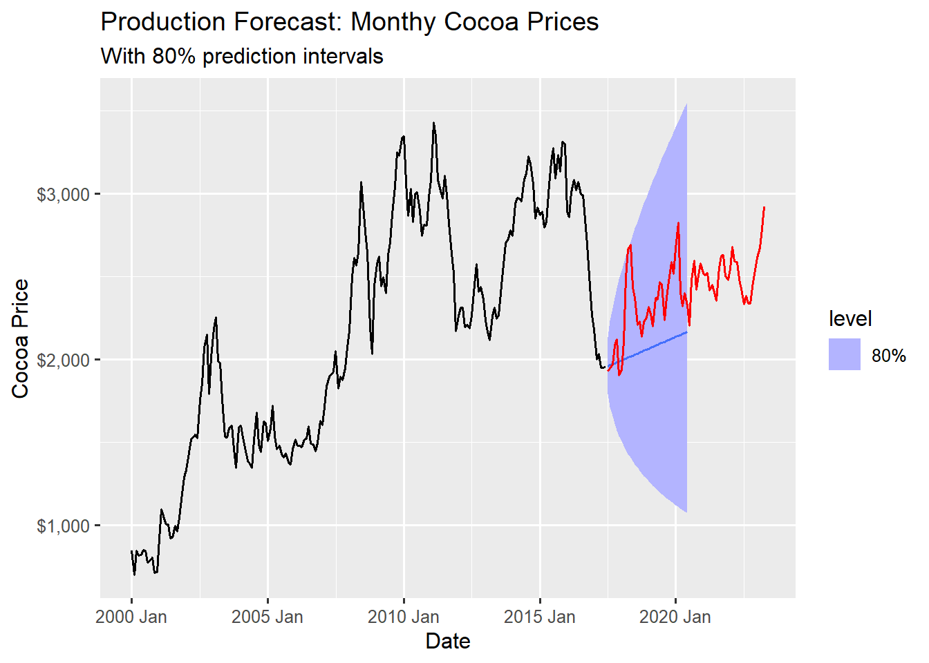
For visualisation purposes, we generate a 3-year forecast (extending beyond the 12-month target). The training history (black line), the forecast (blue line) and the held out test data (red line) are overlayed together on the same plot with an 80% PI (less conservative interval for visual communication). This allows stakeholders to immediately see how well the model would have performed on the most recent history.
17.5.5 Building a Validated Forecasting System
The ultimate goal is to consolidate the entire process into a reusable, self-contained function that can be run automatically (e.g monthly) and generates a complete report and saves the output. For this cocoa prices workflow, a custom function (forecasting_pipeline) has been created as a reference to build your own workflow pipeline. The function can be found here.
Function Logic:
The function simplifies the model selection by training a subset of good models (
ets,arima,s_naive) and selecting the winner based on the lowest MASE calculated internally on the training set.It then calculates the specific point forecast (next period, mid-term average, long-term average), extracts the model details using the
report()function, formats the output into a single string summary, and saves the full data to a.csvfile.
This entire pipeline ensures that the forecast is traceable, validated against historical errors and presented in a format immediately useful for business decision.
17.6 Final Validation Against Test Period
This is the single most important step in the forecasting workflow. It measures how the model, selected through the rigorous cross-validation, performs on data it has never encountered before (the held out testing set; testing_cocoa). This provides the most honest and realistic estimate of the model’s true predictive capability.
For the test validation, we focus on the top two models (arima_log and arima_seasonal) from the cross validation combined rank.
# test set evaluation
test_predictions <-  cocoa_model_portfolio |>
  select(arima_seasonal, arima_log) |>
  forecast(new_data = testing_cocoa)

test_accuracy <- test_predictions |>
  accuracy(cocoa_ts)
The top two models are isolated from the full fitted model portfolio and then instructed to make predictions for the exact time periods defined in the testing_cocoa data as defined in this line of code “forecast(new_data=testing_cocoa)”. The accuracy compares the generated forecasts against the actual prices in the full historical data (cocoa_ts) that spans the training and testing periods.
17.6.1 Comparing Training and Testing Performance
We combine the training and testing accuracy metrics into one table to analyse the generalisation gap – the difference between how well the model fits the past versus how well it predicts the future.
# A tibble: 4 × 6
  .model          MASE  RMSE  MAPE   MAE type
  <chr>          <dbl> <dbl> <dbl> <dbl> <chr>
1 arima_log      0.267  134.  5.00  103. training
2 arima_seasonal 0.265  134.  5.02  102. training
3 arima_log      0.832  362. 12.8   320. testing
4 arima_seasonal 0.659  299. 10.1   254. testing
In both models, the error metric increased significantly from training to testing. For arima_seasonal, \(MAE\) jumped from $102 to $254, and \(MASE\) jumped from 0.265 to 0.659. This increase is expected and normal in forecasting, reflecting the difficulty of predicting the future compared to fitting the past.
On the unseen data, the arima_seasonal model proved substantially superior, its \(MASE\) of 0.659 means the forecast error was 34.1% better than the seasonal naive baseline. Its \(RMSE\) of ~299 was ~$69 lower than the arima_log model, confirming it performed better at avoiding large errors.
The arima_seasonal model as we rightfully selected is therefore suitable for operational deployment due to its strong performance on the robust cross-validation combined with its lowest error on the final testing set.
17.7 Summary
This chapter teaches a complete production-ready time series forecasting workflow using Ghana cocoa prices data as a case study. The core insight is to never trust a single model; always build diverse a portfolio (ETS, ARIMA, NAIVE etc) and use time series cross validation to robustly evaluate performance across time. Equally crucial is quantifying uncertainty through prediction intervals – showing forecast ranges rather than single numbers prevent dangerous overconfidence and helps, stakeholders make informed decisions under uncertainty.
For real world deployment monitor continuously for model decay (retrain if MAPE degrades >50%) and prefer simplicity over marginal complexity – if a complex model improves accuracy by less than 10%, stick with the simpler one. Ultimately, forecasting is not about being perfectly right, but about providing useful, honest predictions that respect uncertainty, critical for decision making and risk management.
17.8 Becoming a Forecasting Practitioner
Congratulations!🎊You have made it to the end of your forecasting journey. Here are some key principles to carry forward;
- Start Simple: Always begin with benchmark models. Complexity should earn its place through demonstrated improvement.
- Embrace Uncertainty: Forecasts are probabilistic by nature. Always communicate prediction intervals and assumptions.
- Validate Rigorously: Use time series cross-validation and hold out tests to avoid self deception.
- Think in Portfolios: Different models serve different purposes maintain a diverse toolkit.
- Monitor continuously: Models decay as patterns change. Implement ongoing performance tracking.
- Communicate clearly: Technical accuracy means nothing if stakeholders do not understand and trust forecasts.
Always remember that forecasting is both science and art. The technical skills you have learnt in this book provides the foundation, but judgement, context awareness and communication turn forecasts into actionable insights. Continue practising with different datasets, stay curious about new methods and always maintain healthy scepticism about your predictions.
The future may be uncertain, but with these skills you are now equipped to face that uncertainty with confidence and competence💪🏽.